Making Cleveland in 50 Maps, Street Designations

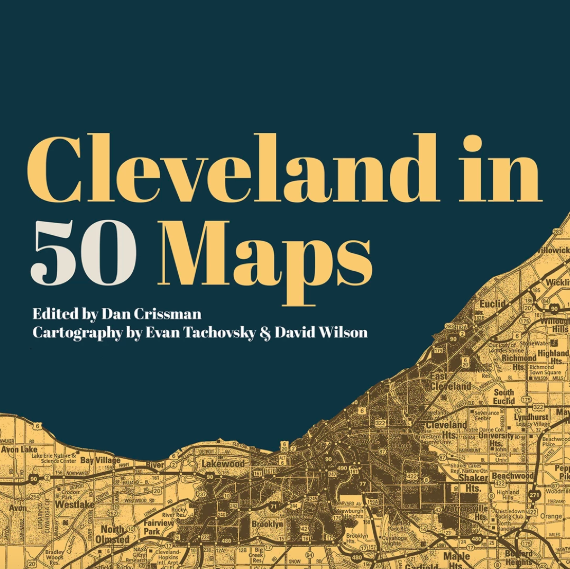
I’m pleased to announce that on October 15, I’ll launch my first book titled Cleveland in 50 Maps with Belt Publishing. I spent the last seven months working on this project with editor Dan Crissman and designer David Wilson. We set out to map how this often misunderstood, caricatured, or simply overlooked region really looks and feels. Thanks in large part to Dan’s and David’s deft touch, I’m really proud of how it turned out.

On the technical side, I made each of the over 50 maps (yes there are bonus maps!) using open source tools. The majority were done in R and with bits of Python, QGIS, and GDAL for data munging.

Over the next few months, I’m going to blog through how I made each map and share the code for anyone to reuse or adapt for their city. Today I’ll start with one of the more straightforward examples: mapping street designations across Cleveland.

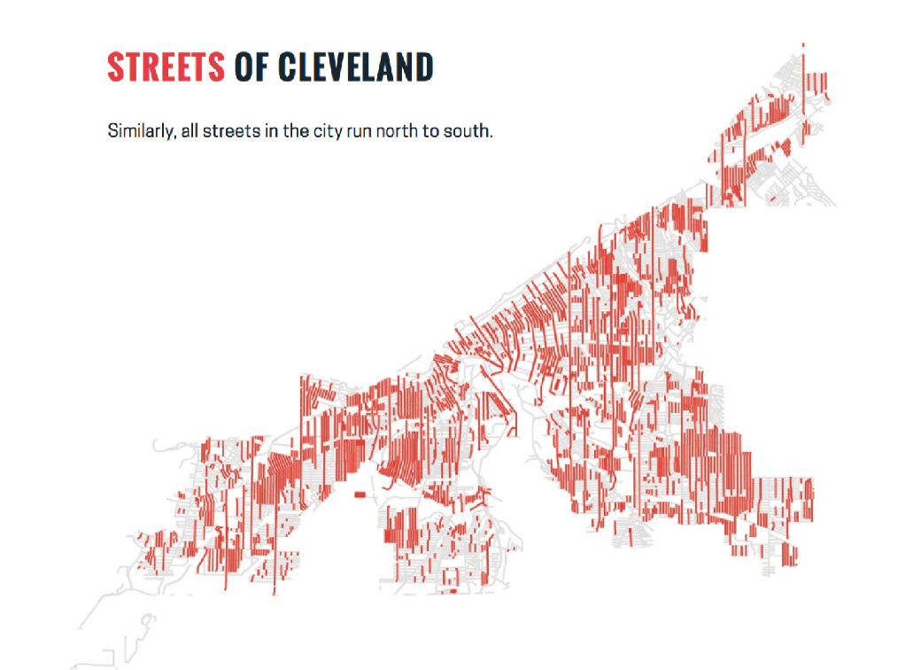
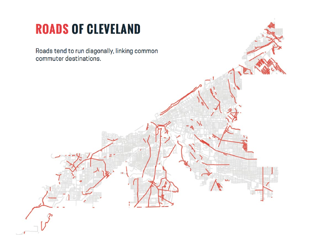
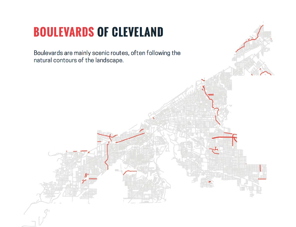
Cleveland’s current street designation system was adopted in 1905 to simplify navigation. Avenues run East-West, streets run North-South and so on. While the system makes sense, there’s something quixotic about trying to apply a grid to a city with such wonky borders and watersheds. More than a few Clevelanders I know were surprised to see the pattern.

There are 23 different designations in Cleveland from the standard “street” or “road” to the quaint “mews” or the eponymous “circle”. For the book, we settled on a set of four maps above (streets, avenues, roads, and boulevards) laid out on sequential pages.

Here’s the code:

## start by loading up the two libraries i used for nearly every map in the book
library(tidyverse)
library(sf)

## to build these maps we'll use data from the Cuyahoga County Open Data portal

# municipal boundaries: https://data-cuyahoga.opendata.arcgis.com/datasets/cuyahoga-county-municipalities/
cle <- read_sf("munis_in_cuyahoga.geojson") %>% 
  # filter down to cleveland boundaries
  filter(MUNI_NAME == "Cleveland")

# roads: https://data-cuyahoga.opendata.arcgis.com/datasets/lbrs-streets-in-cuyahoga-county
roads <- read_sf("cuy_roads.geojson") %>%
  # just roads within the cleveland boundary
  st_intersection(., cle) 

# function that creates and exports a map based on a given suffix
road_mapR <- function(suffix) {

  roads_clean <- roads %>%
    # add a new variable to highlight a given type of street
    mutate(road_highlight = ifelse(STR_SUFFIX == suffix, TRUE, FALSE)) 
  
  road_map <- ggplot() +
    geom_sf(data = roads_clean, aes(fill = road_highlight, color = road_highlight)) +
    scale_fill_manual(values = c("grey90", "#dc6252"), guide = FALSE) +
    scale_color_manual(values = c("grey90", "#dc6252"), guide = FALSE) +
    theme_void(base_family = "mono", base_size = 20) +
    labs(title = glue::glue("{suffix}s in Cleveland, Ohio")) +
    coord_sf(datum = NA)
  
  # use glue::glue to insert the correct suffix in the file name
  ggsave(filename = glue::glue("infrastructure_{suffix}.png"), 
         road_map,
         width = 8, 
         height = 6)
  
}


# pick the four designations of interest
map(c("ST", "AVE", "RD", "BLVD"), road_mapR)

# or map it over all designations
map(unique(roads$STR_SUFFIX), road_mapR)

From a design perspective, I like that the maps look like perturbed bar codes–a sort of fingerprint of the city. After we sent this to the printer, I came across the amazing work of Erin Davis, who took a different design approach to the same problem. It will be well worth your time to check out her work.

One note: the code above produces a set of pngs, which are great for sharing online or in a blog post like this. For the book, I generated svgs and handed them over to David who added the custom fonts and styling touches that made the project book-worthy.