The Bing Maps team at Microsoft recently released a dataset of nearly 125 million building footprints across United States.
These footprints were derived using a two-step process. First, the team used a deep residual neural network to identify likely building pixels. Second, they developed a novel method for grouping the building pixels into sensible polygons.
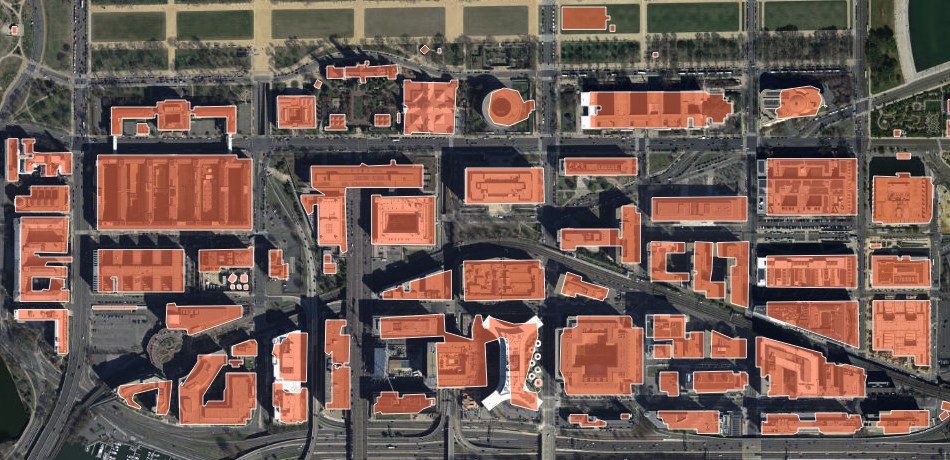
I plotted the building footprints around Mall in Washington, D.C. over satellite imagery for a quick visual inspection:
Spend a few minutes exploring the map and you’ll see (1) that the Bing Maps team’s results are quite good and (2) there are still anomalies that demonstrate why this is such a hard problem. Notably, the two-step approach struggles with irregular buildings, especially those with curves.
Edge cases aside, these are promising results and boon for projects like Open Street Map. I look forward to seeing if/when the Bing Maps team releases datasets for other countries. Those data would be quite helpful for a number of development and humanitarian problems from poverty estimation to disaster response.
The code to download the Microsoft data and build the map is below. As an aside, I recently made the jump and switched my R spatial workflow over from sp to sf. It’s been great and I honestly haven’t looked back once.
library(tidyverse)
library(sf)
library(tigris)
library(mapview)


# download and unzip data from https://github.com/Microsoft/USBuildingFootprints
url_dc <- "https://usbuildingdata.blob.core.windows.net/usbuildings/DistrictofColumbia.zip"
download.file(url_dc, "DistrictofColumbia.zip")
unzip("DistrictofColumbia.zip")

# read in building shapes
dc_buildings <- st_read("DistrictofColumbia.json")

# use the tigris package to get the census tract shapefile
options(tigris_class = "sf") # defaults to sp; manually set to sf
dc_tracts <- tracts(state = "DC")

# filter down to census tracts around the mall
mall_tracts <- dc_tracts %>%
  filter(NAME %in% c(56, 58, 59, 62.02,  65, 66, 82, 101, 102, 105, 107, 108))

# reproject the mall_tracts
mall_tracts_t <- st_transform(hirsh_tracts, st_crs(dc_buildings))

# clip buildings file to just mall_tracts boundaries
dc_building_select <- st_intersection(mall_tracts_t, dc_buildings)

# make a quick interactive map for inspection
mapview(dc_building_select,
        col.regions = "coral",
        color = "white",
        map.type = "Esri.WorldImagery")